Parallel computing refers to the process of breaking down larger problems into smaller, independent, often similar parts that can be executed simultaneously by multiple processors communicating via network or shared memory, the results of which are combined upon completion as part of an overall algorithm.
Example: Estimate \pi
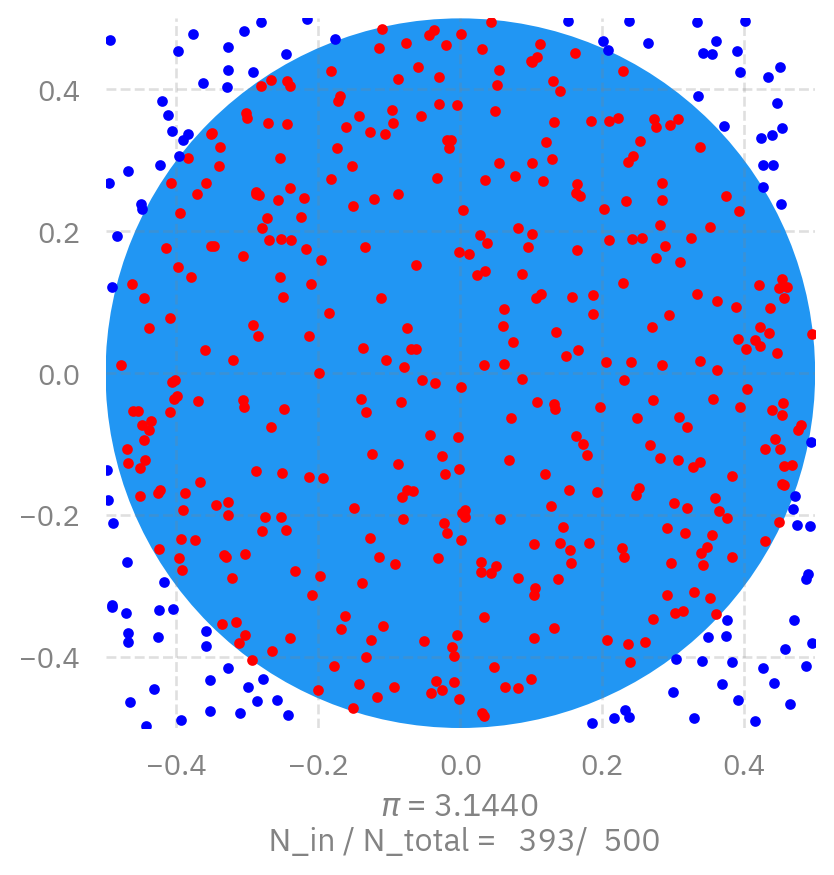
We can calculate the value of \pi using a MPI parallelized version of the Monte Carlo method. The basic idea is to estimate \pi by randomly sampling points within a square and determining how many fall inside a quarter circle inscribed within that square.
\pi
The ratio between the area of the circle and the square is
The parallel computing in AI is usually called distributed training.
Distributed training is the process of training I models across multiple GPUs or other accelerators, with the goal of speeding up the training process and enabling the training of larger models on larger datasets.
There are two ways of parallelization in distributed training.
Data parallelism:
Each worker (GPU) has a complete set of model
different workers work on different subsets of data.
Model parallelism
The model is splitted into different parts and stored on different workers
Different workers work on computation involved in different parts of the model
Figure 1: PI
Figure 2: 3D LLM
Citation
BibTeX citation:
@online{foreman2025,
  author = {Foreman, Sam and Foreman, Sam and Zheng, Huihuo},
  title = {Example: {Approximating} \$\textbackslash Pi\$ Using {Markov}
    {Chain} {Monte} {Carlo} {(MCMC)}},
  date = {2025-07-15},
  url = {https://saforem2.github.io/hpc-bootcamp-2025/00-intro-AI-HPC/5-mcmc-example/},
  langid = {en}
}
---title: 'Example: Approximating $\pi$ using Markov Chain Monte Carlo (MCMC)'description: 'Simple example illustrating how to estimate $\pi$ (in parallel) with Markov Chain Monte Carlo (MCMC) and MPI'categories: - ai4science - hpc - llm - mcmctoc: truedate: 2025-07-15date-modified: last-modifiedformat: ipynb: default-image-extension: svg html: default gfm: toc: trueauthor: - id: sf name: Sam Foreman orcid: 0000-0002-9981-0876 email: foremans@anl.gov affiliation: - name: '[ANL](https://www.anl.gov/)' city: Lemont state: IL url: https://alcf.anl.gov/about/people/sam-foreman - id: hz name: Huihuo Zheng # orcid: 0000-0002-9981-0876 email: huihuo.zheng@anl.gov affiliation: - name: '[ANL](https://www.anl.gov/)' city: Lemont state: IL url: https://alcf.anl.gov/about/people/huihuo-zheng---[](https://colab.research.google.com/github/saforem2/intro-hpc-bootcamp-2025/blob/main/docs/00-intro-AI-HPC/5-mcmc-example/index.ipynb)[](https://github.com/saforem2/intro-hpc-bootcamp-2025/blob/main/docs/00-intro-AI-HPC/5-mcmc-example/README.md)<!--<p> <a href="https://colab.research.google.com/github/saforem2/intro-hpc-bootcamp-2025/blob/main/content/00-intro-AI-HPC/8-clustering/index.ipynb"> <img src="https://colab.research.google.com/assets/colab-badge.svg" class="img-fluid"> </a> <a href="https://github.com/saforem2/intro-hpc-bootcamp-2025/blob/main/docs/00-intro-AI-HPC/5-mcmc-example/README.md"> <img src="https://img.shields.io/badge/-View%20on%20GitHub-333333?style=flat&logo=github&labelColor=gray.png" class="img-fluid"> </a></p>-->::: {.callout-important title="Parallel Computing" collapse="false"}**Parallel computing** refers to the process of breaking down larger problemsinto smaller, independent, often similar parts that can be executedsimultaneously by multiple processors communicating via network or sharedmemory, the results of which are combined upon completion as part of anoverall algorithm.:::## Example: Estimate $\pi$We can calculate the value of $\pi$ using a MPI parallelized version of theMonte Carlo method.The basic idea is to estimate $\pi$ by randomly sampling points within a squareand determining how many fall inside a quarter circle inscribed within thatsquare.The ratio between the area of the circle and the square is$$\frac{N_\text{in}}{N_\text{total}} = \frac{\pi r^2}{4r^2} = \frac{\pi}{4}$$Therefore, we can calculate $\pi$ using $\pi = \frac{4N_\text{in}}{N_\text{total}}$```{python}import ambivalentimport matplotlib.pyplot as pltimport seaborn as snsplt.style.use(ambivalent.STYLES['ambivalent'])sns.set_context("notebook")plt.rcParams["figure.figsize"] = [6.4, 4.8]from IPython.display import display, clear_outputimport matplotlib.pyplot as pltimport numpy as npimport randomimport timeimport ezpzfrom rich importprintfig, ax = plt.subplots()#ax = fig.add_subplot(111)circle = plt.Circle(( 0. , 0. ), 0.5 )plt.xlim(-0.5, 0.5)plt.ylim(-0.5, 0.5)ax.add_patch(circle)ax.set_aspect('equal')N =500Nin =0t0 = time.time()for i inrange(1, N+1): x = random.uniform(-0.5, 0.5) y = random.uniform(-0.5, 0.5)if (np.sqrt(x*x + y*y) <0.5): Nin +=1 plt.plot([x], [y], 'o', color='r', markersize=3)else: plt.plot([x], [y], 'o', color='b', markersize=3) display(fig) plt.xlabel("$\pi$ = %3.4f\n N_in / N_total = %5d/%5d"%(Nin*4.0/i, Nin, i)) clear_output(wait=True)res = np.array(Nin, dtype='d')t1 = time.time()print(f"Pi = {res/float(N/4.0)}")print("Time: %s"%(t1 - t0))```### MPI example| Nodes | PyTorch-2.5 | PyTorch-2.7 | PyTorch-2.8 || :----:| :---------:| :---------:| :---------:|| N1xR12 | 17.39 | 31.01 | 33.09 || N2xR12 | 3.81 | 32.71 | 33.26 |```{python}from mpi4py import MPIimport numpy as npimport randomimport timecomm = MPI.COMM_WORLDN =5000000Nin =0t0 = time.time()for i inrange(comm.rank, N, comm.size): x = random.uniform(-0.5, 0.5) y = random.uniform(-0.5, 0.5)if (np.sqrt(x*x + y*y) <0.5): Nin +=1res = np.array(Nin, dtype='d')res_tot = np.array(Nin, dtype='d')comm.Allreduce(res, res_tot, op=MPI.SUM)t1 = time.time()if comm.rank==0:print(res_tot/float(N/4.0))print("Time: %s"%(t1 - t0))```### Running $\pi$ example on Google Colab* Go to https://colab.research.google.com/, sign in or sign up* "File"-> "open notebook"* Choose `01_intro_AI_on_Supercomputer/00_mpi.ipynb` from the list```{python}#| output: false! wget https://raw.githubusercontent.com/argonne-lcf/ai-science-training-series/main/01_intro_AI_on_Supercomputer/mpi_pi.py! pip install mpi4py``````{python}! mpirun -np 1--allow-run-as-root python mpi_pi.py``````{python}! mpirun -np 2--allow-run-as-root --oversubscribe python mpi_pi.py``````{python}! mpirun -np 4--allow-run-as-root --oversubscribe python mpi_pi.py```### Running $\pi$ on Polaris```bashssh<username>@polaris.alcf.anl.govqsub-A ALCFAITP -l select=1 -q ALCFAITP -l walltime=0:30:00 -l filesystems=home:eagle# choose debug queue outside of the class# qsub -A ALCFAITP -l select=1 -q debug -l walltime=0:30:00 -l filesystems=home:eaglemodule load conda/2023-10-04conda activate /soft/datascience/ALCFAITP/2023-10-04git clone git@github.com:argonne-lcf/ai-science-training-series.gitcd ai-science-training-series/01_intro_AI_on_Supercomputer/mpirun-np 1 python mpi_pi.py # 3.141988, 8.029037714004517 smpirun-np 2 python mpi_pi.py # 3.1415096 4.212774038314819 smpirun-np 4 python mpi_pi.py # 3.1425632 2.093632459640503 smpirun-np 8 python mpi_pi.py # 3.1411632 1.0610620975494385 s```## Parallel computing in AIThe parallel computing in AI is usually called distributed training.Distributed training is the process of training I models across multiple GPUsor other accelerators, with the goal of speeding up the training process andenabling the training of larger models on larger datasets.There are two ways of parallelization in distributed training.* **Data parallelism**: - Each worker (GPU) has a complete set of model - different workers work on different subsets of data. * **Model parallelism** - The model is splitted into different parts and stored on different workers - Different workers work on computation involved in different parts of the model::: {#fig-parallel-computing}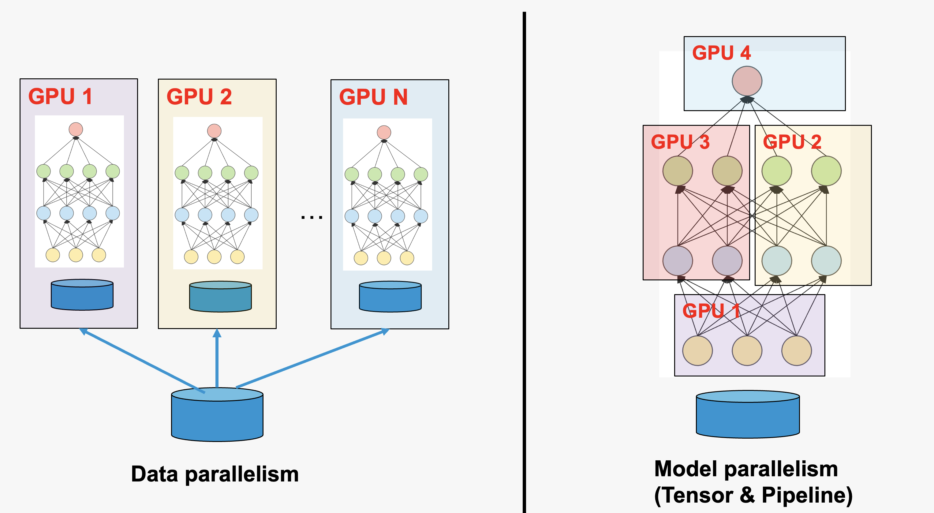PI::::::{#fig-3dllm}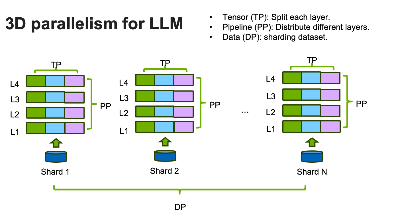3D LLM:::